
# Neural Networks for Non Math People
If you are like me, math may not have been your strongest subject growing up. In fact, I failed pre-calculus two times (proudly passed with a D the third time around - shout out palm beach community college). This lack of foundation made delving into machine learning beyond the conveniently packaged inference api's of open ai or claude feel like a sisyphean task. In this article i will try to explain, to the best of my current understanding, how a basic feed forward neural network works, it's significance relative to the greater state of 🤖gEnErAtIvE Ai🤖 and some resources for gaining a better understanding of their mathematical underpinnings for those interested in learning more.
What it is
Machine learning is a field that belongs sandwiched inside the ven-diagram of engineering and data science. It is all about solving problems with algorithms that learn from data. In the field there are three prevailing approaches: reinforcement learning, supervised learning and unsupervised learning.
In supervised learning you "train" a model (in our case the model is a type of neural network) by using true and false labels. This is usually done by splitting your data up into testing and training sets. The process of training is all about looping through different training examples to figure out how wrong your model's predictions are by calculating something called a gradient and then using that gradient to figure out which way to adjust the model's weights and biases in order to minimize the error. Gradients are important, we will touch on them down below.
Reinforcement is all about solving problems by finding the best policy - there is no true or false labeled dataset to help you minimize an error. Your model interacts with an environment where it receives feedback in the form of rewards (positive) and penalties (negative) in order to find the best policy. An example of reinforcement learning is the n-armed bandit model or e-greedy model. Both are rad.
Unsupervised learning, is where your model learns the labels of your dataset as you train it. It is often used when you want to "cluster" things, which means grouping them together - often by commonality. An example of unsupervised learning is the k-means algorithm, which groups data by clusters in a geometric space.
In modern systems these different paradigms of learning are often used interchangeably. For example, deep reinforcement networks are a promising area of research where supervised learning models are trained in a supervised fashion. Then at the end of training, they are fine-tuned with reinforcement learning methods.
Our focus for this article is getting a basic understanding of one type of supervised learning algorithm, feed forward neural networks.
What is a neural network
A neural network is a supervised learning algorithm that optimizes to minimize the error between a predicted value and an actual value. Depending on the design of it (also known as the "model's architecture"), it accepts an input and learns to classify things or does regression to estimate things. Like an onion or an ogre, it has layers. The layers are where the magic happens. These layers usually contain big lists of lists of floating point numbers e.g.: $[[0.00203...]]$, these lists of lists of numbers are known mathematically as matrixes, although in this context - we call them the weights of the network. I like to think of them visually as a big grid of data. In addition to weights, there are also biases which are also matrixes of numbers. Weights and biases get combined and passed into special functions known as activation functions that control an output.
You may have connected that the prefix neural alludes to the brain. If we model our network as a graph quickly it will make sense why.
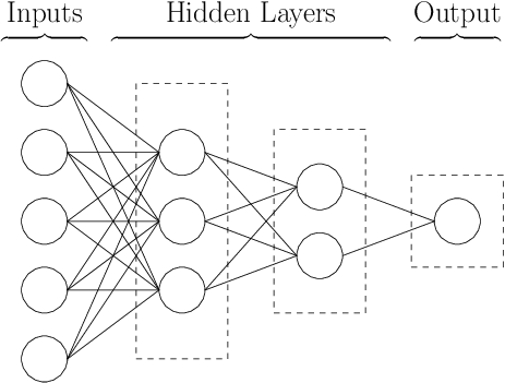
The columns of circles are layers, the layer's circles are our neurons. The neurons are not actually circles in code but really are functions that take an input and combine it with weights and a bias, then apply an activation function to it. The neurons (or functions) of the first layer connect to the layers of the next layer, in this case going left to right (although depending on the architecture of the network, they might go in a different direction too). In the example network we are describing, we have an input layer - two hidden layers, and an output layer.
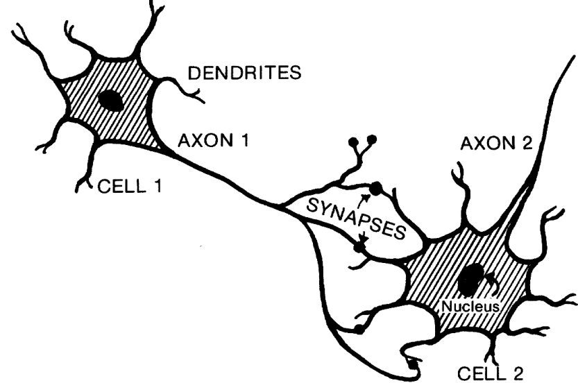
This is kinda like a brain - where you have neurons that have axons and dendrites. They are connected to each other and send data in different directions.
The neurons of our layers perform an operation called an affine transformation, the equation for this looks like this: $$y = Wx + b$$ $W$ is the Weights of the current layer, $x$ is the weight matrix we pass in from our data, $b$ is the bias matrix.
After we have $y$ we put it into something called an activation function, for example, a rectified linear unit or RELU function.
$$ activation = relu(y) $$
Activation functions are important, their job is to decide what shape a neuron's output can be. Depending on the layer of the network we are on (an output layer or a hidden one) there are different types of activation functions you can use. If we are classifying 10 different things, your network's output layer will probably spit out 10 different values - one for each class. Then your activation function turns those raw values into probabilities that all add up to 1, so you can say for a given class "boulder", what is the probability that some input, maybe an image, is a boulder (out of 100%).
The activation function I just described is called a softmax activation function, its famous - but not in an annoying pretentious kind of way.
Lets back up for a second. You now have a very basic understanding of one type of neural network. This is called a feed forward neural network. Historically, it is a very important architecture. It reinvigorated interest in a field that was mislabeled as overpromising. The first networks only had one layer, these were called single layer perceptrons and they were devised in the 40's. They kinda sucked. They were able to learn to separate data that was linearly divided on an $x/y$ graph to split them into categories, they did this by estimating a line called a hyperplane - bit of an aggrandizing title. Stuff that was on one side of the hyperplane was one class and on the other side a different class. When researchers later found out that you could connect perceptrons together into networks of "multi-layer perceptrons", the use cases for neural networks expanded because they were no longer limited to solving linear problems.
Whats actually happening
our architecture:
Our model will have one input layer, two hidden layers and an output layer. Our activation functions we will be applying the non linear relu activation function on both affine transformations of our hidden layers - we will describe why in a second.
For our example, training happens inside of two nested loops.
for thing in loop_1:
	 for thing in loop_2:
		 do something
When the inner loops finishes running the outer loop iterates (runs) one time. During training our outer loop is iterating through what are called epochs and our inner loop is iterating through our training data. Epoch is a fancy word, but it is describing a full loop of the training data. This may help you understand.
for epoch in epochs: (outer loop)
	for batch in training_data_batches: (inner loop)
		Train my model (do something)
Every batch is an instance of training data. Big models like Chat GPT are trained on incomprehensibly large sets of data, this is why in production settings, the work of training is parallelized or distributed across multiple machines happening in unison. The evolution of the graphics processing unit (GPU) made training huge models possible because the operations for rendering graphics also needed to be parallelized and could not run sequentially on a computers central processing unit (CPU) which cannot execute large numbers of operations in parallel.
> That's why NVIDIA is worth so much money and Taiwan semiconductor manufacturing company remains one of the most important companies on the planet.
Lets step back for a second, we are inside of our two loops
network = InitializeModel() # You don't initialize your network every time
for epoch in epochs:
	for batch in training_data_batches:
		You are here -> Train my model
What happens?
Four things!
Data  →  Forward Pass → Prediction → Loss → Backward Pass → Updated Weights
             |                                                ↑
             └──────────────────── Training Loop ─────────────┘
-
Initialization of the model - def init(): Technically this happens above the two loops, but i wanted to include it. You make or initialize your network with some basic descriptions of what your input looks like and what your output should look like. These details are called hyper parameters and they include learning rates, seed's for random number reproducibility, hidden_layer size, output layer size and input layer size. We will also initialize our weights and biases. The way we initialize our weights and biases matters. Everything is connected, so if you pick the wrong initialization strategy for your activation function - training can stall.
-
Forward propagation of the model - def forward(X): After you initialize your model with its hyper parameters, the forward pass of the network takes the weights and biases you initialized - as well as a matrix containing your training data (X) to make a prediction. In our example, we are training a network to predict the popularity of wine based on a feature set containing information about it. It is a regression problem, because we are taking a bunch of numeric values and regressing to a single score (Which is also a number). Technically you could solve this with plain old linear regression, however, non linear methods will help us find "latent" (important word, come back to in a second) connections between our data's features and get a better performing model. Again, performance in this case is measured by us training a generalizable model that has a low error rate or difference between the actual value and the predicted value.
Following up on forward propagation, the code implementation of this looks something like this.
class Network:
	def __init__(self, input_size, hidden_size, output_size):
		seed = 0.005

		self.W1 = np.random.randn(input_size, hidden_size) * seed #random seed
		"""
		 ^ This generates our first layer's weights, a matrix of random numbers.
		 Don't get thrown off by the code here, np (numpy) is a popular library for data science and ml. It uses c under the hood to work a lot faster than normal python. There are a ton of really conveinent linear algebra and calculus functions built in. I digress.
		"""
		self.b1 = np.zeros(hidden_size, hidden_size)
		"""
		Initialize bias matrix
		"""
		self.W2 = np.random.randn(hidden_size, hidden_size) * seed
		# Same thing but layer 2
		self.b2 = np.zeroes(hidden_size, output_size)

	def forward(self, X) -> Dict:
		z1 = np.dot(X, self.W1) + self.b1 # Remember our Wx+b affine function!
		a1 = relu(z1) # Here it is!
		z2 = np.dot(a1, self.W2) + self.b2
		y_hat = relu(z2)
		cache = {'z1': z1, 'a1':a1, 'z2':z2, 'y_hat': y_hat}
		return cache
Okay, that was some code i just through at you. I'd like to formally apologize if you weren't expecting it. However, the idea of code is way scarier than whats actually going on.
def __init__ is called a python constructor function, you will see it all over the place - it's a cool language, worth learning a little bit of. When you define a class in python you are kind of designing a skeleton for a type of object you want to create in memory. When you initialize or create a new instance of a class python calls the constructor function and it initializes whatever instructions you give it. You'll notice the word self a lot too. That just refers to a specific instantiation of an object of that class. So in english, if i say network1 = Network(input_size, hidden_size, output_size), network1's constructor get's called and creates those W1 b1 ,etc variables on the object depending on what input_size, hidden_size, and output_size are.
Back to the ml - We have created our model, network1, with some random weights and biases. It knows nothing, hasn't seen any data, has no knowledge - we must make it learn. To do that, we need it to tell us how little it knows about its task of predicting wine score. No one starts off as an expert, that's true for neural networks too. Thats where the forward pass comes in! For the type of model we are training, our forward passes returns a series of variables about the prediction, including all the intermediate steps it took to get to the point of actually having y_hat, which is our prediction. I call this y_hat because in math the hat in this context means a predicted value.
The importance of gradients in back propagation
An interesting thing happened in the 80's in neural networks. Three researchers popularized an approach for improving models performance in a substantial way. At this point, multi layer perceptron algorithms had been established. Networks were able to contain multiple layers, however - the way that they learned was limited. Multi layer perceptron's could do a forward pass and make predictions but there was no way to find out how individual neurons contributed to the total error and how to update them in order to correct that error. That's like saying you are running a software company, someone in your organization keeps releasing changes that break production, you have no system to find that person and help them improve their performance.
Enter in back propagation,
The back propagation algorithm tracks how each layer contributed to the overall loss (or error) of the networks prediction. It does this backwards, starting from the outermost layer and going inwards through all of your networks layers. forward pass goes forward, backward propagation goes backward. It relies on some multivariable calculus, namely something called the chain rule - and partial derivatives to create whats called a gradient that it uses to descend and try to find a global minimum.
To recap, a derivative measures how a function changes over time. A partial derivative measures how a function changes over time with respect to a specific variable. If we think about our problem again, our neurons are functions, we want to know how each function contributes to the total cost (or loss) of the models prediction. To find a partial derivative, you need something called the chain rule. In calculus, the chain rule is the way you measure the rate of change of functions that depend on other functions, for example:
function = f(g(x))

where g(x) = X^2
and f(x) = xy
---
af/ag = 2x
af/af = y
---
y(2x)
---
2xy
The chain rule says take the derivative of the inner most function first, then the outermost function with respect to the inner function. Its kind of like our order of operations for taking derivatives of functions that depend on each other.
When we combine a bunch of these partial derivatives into a vector, we have whats called a gradient. For context, this is what a vector looks like in mathematic notation: $\langle 1,2,3 \rangle$. If we plot a gradient, it looks something like this:
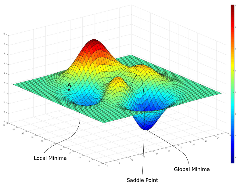
It looks like a mountain, or a hill. In neural networks, we have tons of functions that depend on each other, and sometimes we want to track how multiple outputs change at once.
> Quick aside, the next section gets a little hairy, at this point you know a little bit about gradients, thats enough - for the adventurous dive in below!
To do that, we go one order higher than the gradient — we use a Jacobian. A jacobian is like a cool older cousin of a gradient, its mature and moved out. It is comprised of the partial derivatives for a vector valued functions, or functions that have many outputs.
We use a reduced form of the jacobian, or specifically a jacobian vector product, to calculate the gradient of the partial derivatives of our weights and biases with respect to our loss function during back propagation as a scalar value (single number). Thats because we only care about how the loss changes with respect to each parameter — not how every output changes individually, which is what a jacobian would give us.
That would be unnecessary and expensive to do in a big training loop a bunch of times, I only bring it up here because what we are doing when we return multiple gradients together from our back propagation function borrows conceptually from the jacobian. I hope that wasn't needlessly confusing, if it was i'm sorry - stuff will make more sense in a second.
> End of my math rant.
Lets look at some code.
- Back propagation of the model - def backward(X):
def backprop(self, X, cache, y):
	a1, b1, b2, y_hat = cache
	m = X.shape[1]

	# Derivative of loss wrt output (for MSE)
    dL_dyhat = (y_hat - y) / m

    # Output layer gradients
    dL_dW2 = a1.T @ dL_dyhat         # ∂L/∂W2
    dL_db2 = np.sum(dL_dyhat, axis=0, keepdims=True)  # ∂L/∂b2

    # Backprop through hidden layer (ReLU)
    dL_da1 = dL_dyhat @ self.W2.T
    dL_dz1 = dL_da1 * (z1 > 0)       # derivative of ReLU

    # Hidden layer gradients
    dL_dW1 = X.T @ dL_dz1
    dL_db1 = np.sum(dL_dz1, axis=0, keepdims=True)

    # Return all gradients
    gradients = (dL_dW1, dL_db1, dL_dW2, dL_db2)
    return gradients
This is a gnarly one to look at. I'm going to go line by line and explain whats happening.
lines: 1-2
a1, b1, b2, yhat = cache
m = X.shape[1]
Here we are de-structuring our data from our forward propagation. This means we initialize all the variables in scope of our back propagation function. We also instantiate m, which is the number of samples we have in our weight matrix
lines: 3
dL_yhat = (y_hat - y) / m
This line finds the derivative of y_hat, it does so by using a cost function. The cost function we use is Mean squared error - Mean squared error is a common cost function that tells you on average, how wrong your predictions are.
lines: 4-5
dL_dW2 = a1.T @ dL_dyhat         # ∂L/∂W2
dL_db2 = np.sum(dL_dyhat, axis=0, keepdims=True)
We calculate the derivative of the loss with respect to the weights at layer 2 and the bias at layer 2. We start at 2, because back propagation starts at the outermost layer and moves inwards. The @ is a matrix multiplication operator we get from numpy. say we have these matrixes: $[[1,1],[2,2],[3,3]] @ [[1, 1],[1,1]]$ , if we run that operation we get this: $$[[2,2],[4,4],[6,6]]$$
So we multiply the transpose (flipped) matrix of our first affine transformation by the derivative of our cost function which tells us how much the weights of layer 2 contributed to that error. Then we get the bias with this np.sum thing which sums the bias matrix into a array of 10 elements like this:
l = np.array((64, 10), float)
print(l) ->

array([[0., 0., 0., 0., 0., 0., 0., 0., 0., 0.],
       [0., 0., 0., 0., 0., 0., 0., 0., 0., 0.],
       [0., 0., 0., 0., 0., 0., 0., 0., 0., 0.],
       [0., 0., 0., 0., 0., 0., 0., 0., 0., 0.],
       [0., 0., 0., 0., 0., 0., 0., 0., 0., 0.],
       [0., 0., 0., 0., 0., 0., 0., 0., 0., 0.],
       [0., 0., 0., 0., 0., 0., 0., 0., 0., 0.],
       [0., 0., 0., 0., 0., 0., 0., 0., 0., 0.],
       [0., 0., 0., 0., 0., 0., 0., 0., 0., 0.],
       [0., 0., 0., 0., 0., 0., 0., 0., 0., 0.],
       [0., 0., 0., 0., 0., 0., 0., 0., 0., 0.],
       [0., 0., 0., 0., 0., 0., 0., 0., 0., 0.],
       [0., 0., 0., 0., 0., 0., 0., 0., 0., 0.],
       [0., 0., 0., 0., 0., 0., 0., 0., 0., 0.],
       [0., 0., 0., 0., 0., 0., 0., 0., 0., 0.],
       [0., 0., 0., 0., 0., 0., 0., 0., 0., 0.],
       [0., 0., 0., 0., 0., 0., 0., 0., 0., 0.],
       [0., 0., 0., 0., 0., 0., 0., 0., 0., 0.],
       [0., 0., 0., 0., 0., 0., 0., 0., 0., 0.],
       [0., 0., 0., 0., 0., 0., 0., 0., 0., 0.],
       [0., 0., 0., 0., 0., 0., 0., 0., 0., 0.],
       [0., 0., 0., 0., 0., 0., 0., 0., 0., 0.],
       [0., 0., 0., 0., 0., 0., 0., 0., 0., 0.],
       [0., 0., 0., 0., 0., 0., 0., 0., 0., 0.],
       [0., 0., 0., 0., 0., 0., 0., 0., 0., 0.],
       [0., 0., 0., 0., 0., 0., 0., 0., 0., 0.],
       [0., 0., 0., 0., 0., 0., 0., 0., 0., 0.],
       [0., 0., 0., 0., 0., 0., 0., 0., 0., 0.],
		.... this goes for 64 rows, trust me.

# then if we do the sum on this fake bias matrix
# i just made to illustrate what the sum does.
r = np.sum(l, axis=0, keepdims=True)
print(r)
-> array([[0., 0., 0., 0., 0., 0., 0., 0., 0., 0.]])
print(r.shape)
-> (1, 10)
This sums all the 64 rows into 1 row for each of the 10 columns. So we find out how much layer 2 contributed to the loss and then condense the biases.
Lines 6-7:
Okay we understand how our output layer contributed to how wrong our prediction was, our network has an output layer -> a hidden layer -> and an input layer, so we need to understand what our hidden layer got wrong next.
dL_da1 = dL_dyhat @ self.W2.T
dL_dz1 = dL_da1 * (z1 > 0)
dL_da1 is the same thing that happened above in line 4, matrix multiplication. The W2.T is transposing the weights of W2. and getting the Hadamard product (is the fancy word for it).
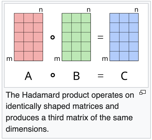
so we flip and multiply, flip and multiply. It gets interesting one line down in dL_dz1 = dL_da1 * (z1 > 0). Here we are getting the derivative of the loss of dz1 by multiplying the derivative of our activation function (derivative of relu is z1 > 0) and multiplying our dL_da1 by it to figure out how much our pre-activation layer 1 contributed to our loss. So we are again walking backward through our chain of functions using the chain rule and derivatives to understand what happened at every step of our networks forward pass.
lines 8-10:
# Hidden layer gradients
dL_dW1 = X.T @ dL_dz1
dL_db1 = np.sum(dL_dz1, axis=0, keepdims=True)

# Return all gradients
gradients = (dL_dW1, dL_db1, dL_dW2, dL_db2)
This is continuing what we did above to create an understanding (in the form of gradients) backwards from our hidden layer to the start of our network at W1 and b1. Then we return everything!
I'm now going to show you guys what these gradients look like plotted out and how they should change, to reiterate this change the shape of gradients reflects our model learning from its mistake.
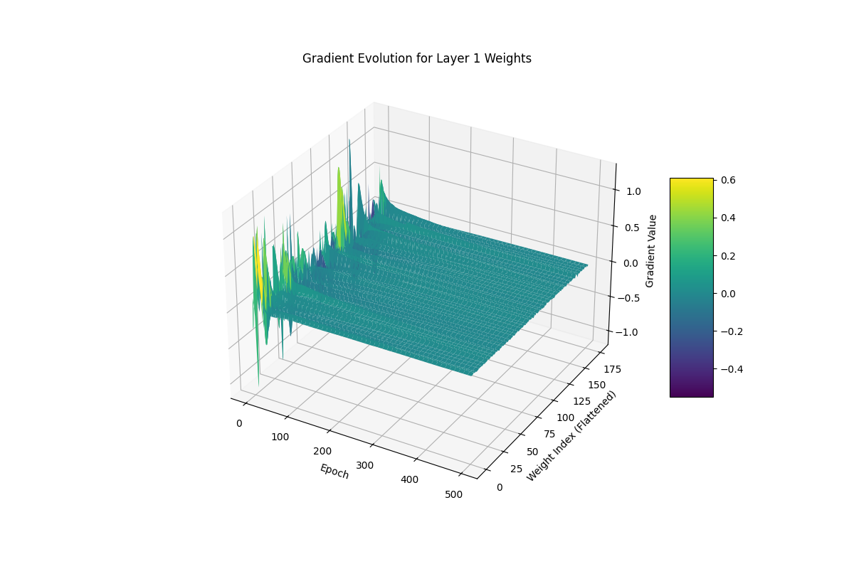
This shows the weights updating over time towards a global minimum and the network learning! It's good to point out that this step technically includes part 4 (the next part) for updating the models weights but i think its a good way to visualize what data you are actually doing to the weights in each iteration of training.
- Updating the model's weights and biases - def update_params(): Updating weights takes the output of our back propagation and the learning rate to do the following. So you multiply the learning rate (how fast you make changes to the weights) by the derivatives you generated in your back propagation algorithm and adjust the weights by those values!
def update_params(self, gradients)
	# Destructure our gradients
	dL_dW1, dL_db1, dL_dW2, dL_db2 = gradients
	self.W1 -= self.learning_rate * dl_dW1
	self.b1 -= self.learning_rate * dl_db1
	self.W2 -= self.learning_rate * dl_dW2
	self.b2 -= self.learning_rate * dl_db2
This is how our network corrects itself and learns. To see the full thing in progress look below:
import numpy as np
import pandas as pd
from sklearn.utils import gen_batches

def relu(n):
	return np.maximum(0, n).astype('float')

class Network:
	def __init__(self, input_size, hidden_size, output_size):
		seed = 0.005
		"""
		 This generates our first layer's weights, a matrix of random numbers.
		 Don't get thrown off by the code here, np (numpy) is a popular library
		 for data science and ml. It uses c under the hood to work a lot faster
		 than normal python. There are a ton of really conveinent linear
		 algebra and calculus functions built in. I digress.
		"""
		self.W1 = np.random.randn(input_size, hidden_size) * seed #random seed
		# Initialize bias matrix
		self.b1 = np.zeros((1, hidden_size))

		# Same thing but layer 2
		self.W2 = np.random.randn(hidden_size, output_size) * seed
		self.b2 = np.zeros((1, output_size))

	def forward(self, x_train) -> tuple:
		"""
		Makes predictions!
		"""
		z1 = np.dot(x_train, self.W1) + self.b1 # Remember our Wx+b affine function!
		a1 = relu(z1) # Here it is!
		z2 = np.dot(a1, self.W2) + self.b2
		y_hat = relu(z2)
		cache = (z1, a1, z2, y_hat)
		return cache

	def backward(self, x_train, cache, y_train):
		z1, a1, z2, y_hat = cache
		m = x_train.shape[0]

		# Derivative of loss wrt output (for MSE)
		dL_dyhat = (y_hat - y_train) / m

		# Output layer gradients
		dL_dW2 = a1.T @ dL_dyhat         # ∂L/∂W2
		dL_db2 = np.sum(dL_dyhat, axis=0, keepdims=True)  # ∂L/∂b2

		# Backprop through hidden layer (ReLU)
		dL_da1 = dL_dyhat @ self.W2.T
		dL_dz1 = dL_da1 * (z1 > 0)       # derivative of ReLU

		# Hidden layer gradients
		dL_dW1 = x_train.T @ dL_dz1
		dL_db1 = np.sum(dL_dz1, axis=0, keepdims=True)

		# Return all gradients
		gradients = (dL_dW1, dL_db1, dL_dW2, dL_db2)
		return gradients

	def update_params(self, gradients, learning_rate):
		# Destructure our gradients
		dL_dW1, dL_db1, dL_dW2, dL_db2 = gradients
		self.W1 -= learning_rate * dL_dW1
		self.b1 -= learning_rate * dL_db1
		self.W2 -= learning_rate * dL_dW2
		self.b2 -= learning_rate * dL_db2

##############################
#### end of network definition
##############################

# Load and prepare data
df = pd.read_csv("winequality-red.csv", sep=";")
X = df.drop("quality", axis=1).values
y = df["quality"].values.reshape(-1, 1)

# Simple normalization
X = (X - X.mean(axis=0)) / X.std(axis=0)

# Define sizes
input_size = X.shape[1]
hidden_layer_size = 64
output_size = 1

batch_size = 32
training_batches = []
for batch_slice in gen_batches(len(X), batch_size):
	x_batch = X[batch_slice]
	y_batch = y[batch_slice]
	training_batches.append((x_batch, y_batch))

# Begin setting up for training
network = Network(
	input_size=input_size,
	hidden_size=hidden_layer_size,  # Fixed: matches __init__ argument
	output_size=output_size
)

# set the learning rate here
learning_rate = 0.001

epochs = 200

# range turns a number into an iterable you can loop through.
for epoch in range(epochs):
	for index, (x_train, y_train) in enumerate(training_batches):
		prediction_cache = network.forward(x_train=x_train)

		# our prediction
		y_hat = prediction_cache[3]

		# calculate loss of the network using mean_squared_error
		# which takes the average of the difference between our
		# prediction and the training example
		# over time to see how it learns.
		loss = np.mean((y_hat - y_train)**2)

		#back propagation
		gradients = network.backward(
			x_train=x_train,
			cache=prediction_cache,
			y_train=y_train
		)

		# Make it learn!
		network.update_params(
			gradients=gradients,
			learning_rate=learning_rate
		)

		# at the end of every training batch per epoch print
		# the loss to track learning
	if epoch % 10 == 0:
		print(f'epoch: {epoch}; loss {loss:.4}')
Next time we will dive into using this network for regression, making predictions of wine scores with it!
BUT WAIT THERES MORE!
For the curious, looking to get a bit more into the weeds i have some recommendations into resources on where you can go to learn about neural networks and deep learning starting from easiest (relatively, all of this stuff is tricky - be kind to yourself) to more advanced, in the weeds books. I've used these for furthering my understanding of the field and plan on continuing to do so. Not claiming if you do all these you'll get a job as a data scientist, hasn't happened to me yet, but you will probably know enough to impress the nerdy side of your family over thanksgiving.
-
Math for Deep Learning - No Starch Press A good introductory book for those needing a refresher on their math skills. Explains linear algebra, bayesian statistics, calculus and multivariable calculus you need to get a grasp on neural networks.
-
Fundamentals of Deep Learning, 2nd Edition – OReilly This is a good resource I had gifted to me from my friend Mauro who is wicked smart! It was a great introductory book into some of the math behind deep learning and i'd recommend it to anyone interested at a beginner level. I think you usually have to pay for this but i think it's worth it!
-
Why Machines Learn - Anil Ananthaswamy A great read for the historical timeline that got us to where we are with AI with a lot of math breakdowns along the way. This book really helped me understand the importance of certain breakthroughs, specifically with back propagation.
-
*Multivariable Calculus Course - MIT OCW This course helped me understand gradients and vectors pretty well, which can get really confusing. It was a great run way to become familiar with different mathematic notations you will see in research papers.
-
Deep learning book - Ian Goodfellow and Yoshua Bengio and Aaron Courville More centered around math used in practice for neural networks, this is a great resource for people interested in seeing the math being used. Totally free, available at https://www.deeplearningbook.org
@book{Goodfellow-et-al-2016, title={Deep Learning}, author={Ian Goodfellow and Yoshua Bengio and Aaron Courville}, publisher={MIT Press}, note={\url{http://www.deeplearningbook.org}}, year={2016} } -
Dive into Deep Learning - D2L.AI I read this one early on, its a textbook - it gets pretty math heavy - i wouldn't say its really easy so i'd go into it with some solid math understanding already built up from some of the previous materials. Great thing is that it's organized and completely free - so if you are really into learning about deep learning, this is a good resource worth checking out. Shout out to Andrew Buchanan for the rec.
-
Pattern classification – David G. Stork, Peter E. Hart, and Richard O. Duda This is one i'm currently working through, it's dense and kind of old, but one of the best math textbooks on pattern recognition there is. I'm reading it and constantly looking things up because it gets kind of gnarly.
-
The Matrix Calculus You Need For Deep Learning – Terence Parr and Jeremy Howard I read this paper after doing my multivariable calculus course - it got gnarly, but also helped me make sense of what happens in a neural network during training. It starts very calculus forward and then ties that into the deep learning stuff at the end nicely. I think its a must read once you have some math confidence.
-
Neural Networks and Deep Learning - By Michael Nielsen / Dec 2019 This is another great free resource that helped me understand neural networks - i found it through the matrix calculus you need for deep learning . It's completely free and totally worth taking a look at. I read up to chapter 3 and need to keep going because its a wonderful free resource.
-
A guide to convolution arithmetic for deep learning - Vincent Dumoulin 1 F and Francesco Visin 2 F This is an awesome look into the math of convolutional neural networks that i just found while writing this article. It was also referenced by Jeremey Howard's page and goes into detail about specific math that makes up pooling and convolutional layers. I'm interested in GNN's which rely a lot on CNN's to understand the topology of a graph, similar to how CNN's can "understand" or classify an image.
-
Reinforcement Learning: An Introduction - Sutton This is a great resource for learning about the exciting field of reinforcement learning. Stanford has a free link to it on it's website . I highly recommend anyone interested in pursuing the field give it a look at least once, it's well written and engaging. Also free - free education is nice!
Paid online courses
- Neural Networks and Deep Learning - DeepLearning.AI This is a good course if you have some math and coding skills built up already and want something structured to follow - it has good interviews with some really important and interesting researchers like Geoffery Hinton. I think it's worth $50 if you plan on doing it over the course of a month, i wouldn't start with this though if it's your only exposure to python and math. Great additional reading resources in the courses as well. They also offer an NLP course that has been recommended to me.